Atoms and the Periodic Table V: The Orbitals of Hydrogen Atom
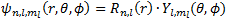
In this section, we will try to sketch the orbitals for the hydrogen atoms based on our wave function that we have split in the previous section. The equation is:
 Then, we can start the discussion from the radial function [R(r)].
The radial function basically describes the possible position of electron with respect to to r (atomic radius). Therefore, if the radius is going to , it means the position is going further away from the nucleus, which less probability to find the electron. Therefore, the radial function is going to 0, as r is going to . Moreover, our system is a bound system which is described as the electron cloud system (ψ2). Hence, we can write the radial function as:
 Before, we draw the radial function of each orbital, we should be able to read our function first. The first part of the function is the rl which describes the area near the origin (nucleus). As the l increases, it means bigger possibility to found the electron near nucleus. Then, the polynomial part describes the number of the nodal point. The last part of the function described the far region of the hydrogen atom and as the r increases the value of R(r) approaches 0. Hence, we can start to draw the function.
We start from the simplest one, 1s orbital. 1s orbital has n=1 and l=0, so the first part is simply r0 which equal a constant. Then, the second part, the polynomial, does not have any nodes. Thus, the graph will not cross the x-axis and the last part will approach to 0. If we move to 2s and 3s orbital, the first and the last part is the same as 1s orbital, but the difference is on the polynomial part. If 1s orbital does not have any radial nodes, 2s orbital will have 1 radial node, and 3s orbital will have 2 radial nodes. We can summarise number of nodes in ns orbital is (n-1) .Therefore the radial function of 1s, 2s, and 3s orbital is:
 Then, in 2p orbital, n = 2 and l = 1, which means rl = r, so the first part of the radial function will be a linear function. In polynomial function, 2p does not have any radial nodes and the last part is similar with s orbital. Generally, the last part of orbital is similar with other orbital (it approaches 0). If we move to 3p and 4p orbital, 3p orbital will have 1 radial node and for 4p orbital will have 2 radial nodes due to polynomial part in the radial function. After p orbital, we also have 3d orbital which have l = 2, the first part become r2, which means increasing faster than p orbital. In 3d orbital, there is no radial node and it will approach 0 as radius increases. The number of radial nodes for p and d orbital is (n-2) and (n-3) respectively. To summarise we can see at the diagram of the radial functions below.
 After we inspects the radial function, we can move to the angular function [Y(θ, ϕ)]. The angular function is related to the shape orbital itself. In s-orbital both l and is ml = 0. Therefore, we can conclude that s orbital is independent to angle, so s orbital is a spherical orbital. A spherical orbital has a consequence that it does not have any angular nodes. Hence, the shape or s-orbital is:
 Moreover, for 2s orbital is shown below. Besides that, you can see as well the radial node of 2s below (a gap between blue and red region).
 For p-orbital, l = 1 which means it has an angular nodes, but p-orbital has 3 values of ml (-1,0,1). The value of describes the different angular momentum for each orbital around z-axis but the same magnitude of momentum (l = 1). The number of ml also means there are 3 different nodal plane for p-orbital, which means x, y, and z are the nodal plane. However, the value of x, y, z are still has dimension, so to make dimensionless it is simply divided with r. Therefore, we have the nodal planes are:
 For example, ml= 0, it does not have momentum around z-axis. Its angular variation is proportional to cos θ. Moreover, if we have px orbital it has the nodal plane is around x-axis and the angular variation is proportional to cos θ, so the value will be positive at x > 0, and x < 0 will have negative value. Therefore, the angular variation at cartesian coordinate is:
 It can also apply for another p-orbital, so the shape of p-orbital is:
 For d-orbital is more complicated than p-orbital because d-orbital has 5 different value of ml (-2, -1, 0, 1, 2). Then, for the nodal plane it has 6 combination (x2, xy, xz, y2, yz,, z2), which d-orbital needs only 5 independent combination which depends on the angle. Based on the experiment, the nodal planes for d-orbital are:
 For the first three nodal planes, it is simply the nodal planes are lie on x, y, or z axis and for example orbital has nodal plane on x and y axis. Therefore, the angular variation is:
 If we apply the same way for the first three orbital we can get the shape as:
 For the 4th orbital which commonly known as dx2-y2 has the nodal planes as x=y and y=-x. Then, the 5th orbital which known as has the angular variation positive at z-axis and the negative makes ring-like structure around the z-axis. Therefore the shape of and is:
 After we can predict the shape of the orbital, we can back to our main problem to find the probability of the electron at given place. As we have discussed previously ψ2 describes the electron distribution at the space or the probability density, and |ψ (r, θ, ϕ)|2 is the probability of electron at space from r to dr, which means the volume of the space between 2 sphere (dV). Therefore, to find dV it can be done with 2 ways, by calculating the difference of volume a sphere with r radius and (r + dr) radius, or by using the general formula of volume an object (Area x height) with the area is the area of sphere with radius r and the height is dr. Both method will find that dV is:
 After that, dV is multiplied ψ2 with as the radial function [R(r)], so we can find the probability of electron at the space. Therefore, the equation is:
 P(r) is basically the probability of the electron to be found at given r. After that, to generate the graph is simply by multiplying R(r)2 with r2 as shown below for 1s and 2s orbital.
 With the same method, we can plot another orbitals as shown below:

From the graphs above, we can spot there are 4 trends on the radial distribution of the orbitals.
1. It form a range of "hills" which represent a high possibility of the electron at given radius. Moreover, the number of "hills" increases as n increases.
2. As the n increases, the highest probability moves to the right side. This shifting represent that higher n, the probability of the electron to be found is going further from the nucleus.
3. At the given n, the radius of the most probable place of electron to be found is d-orbital, p-orbital, and s-orbital (if there is f-orbital it will be the closest one).
rs > rp > rd
4. Although, s-orbital has the biggest radius but it has local maximum that is the closest to the nucleus compare with p and d-orbital. It means the electron sometimes spend closely to the nucleus. This phenomena is called the penetration, which means s is more penetrating to the nucleus compare with the other orbitals.
For more information about the orbitals (the shape, the wave function, the radial distribution, etc.), you can check at the ORBITRON.
The radial function basically describes the possible position of electron with respect to to r (atomic radius). Therefore, if the radius is going to
, it means the position is going further away from the nucleus, which less probability to find the electron. Therefore, the radial function is going to 0, as r is going to . Moreover, our system is a bound system which is described as the electron cloud system (ψ2). Hence, we can write the radial function as:


From the graphs above, we can spot there are 4 trends on the radial distribution of the orbitals.
1. It form a range of "hills" which represent a high possibility of the electron at given radius. Moreover, the number of "hills" increases as n increases.
2. As the n increases, the highest probability moves to the right side. This shifting represent that higher n, the probability of the electron to be found is going further from the nucleus.
3. At the given n, the radius of the most probable place of electron to be found is d-orbital, p-orbital, and s-orbital (if there is f-orbital it will be the closest one).
rs > rp > rd
For more information about the orbitals (the shape, the wave function, the radial distribution, etc.), you can check at the ORBITRON.
Comments